38 remove data labels from excel chart

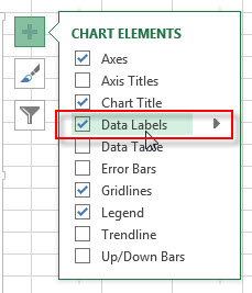
Add or remove data labels in a chart - support.microsoft.com On the Design tab, in the Chart Layouts group, click Add Chart Element, choose Data Labels, and then click None. Click a data label one time to select all data labels in a data series or two times to select just one data label that you want to delete, and then press DELETE. Right-click a data label, and then click Delete. Add / Move Data Labels in Charts - Excel & Google Sheets Double Click Chart Select Customize under Chart Editor Select Series 4. Check Data Labels 5. Select which Position to move the data labels in comparison to the bars. Final Graph with Google Sheets After moving the dataset to the center, you can see the final graph has the data labels where we want.

Excel Chart delete individual Data Labels First select a data label, which will select all data labels in the series. You should see dark dots selecting each data label. Now select the data label to be deleted. This should remove the selection from all other labels and leave the specific data label with white selection dots. Deletion now will remove just the selected data point.

Remove data labels from excel chart

Axis Labels overlapping Excel charts and graphs - AuditExcel.co.za Stop Labels overlapping chart. There is a really quick fix for this. As shown below: Right click on the Axis. Choose the Format Axis option. Open the Labels dropdown. For label position change it to 'Low'. The end result is you eliminate the labels overlapping the chart and it is easier to understand what you are seeing . How to Create a Dynamic Chart Range in Excel The above steps would insert a line chart which would automatically update when you add more data to the Excel table. Note that while adding new data automatically updates the chart, deleting data would not completely remove the data points. For example, if you remove 2 data points, the chart will show some empty space on the right. To correct ... How to hide zero data labels in chart in Excel? - ExtendOffice Sometimes, you may add data labels in chart for making the data value more clearly and directly in Excel. But in some cases, there are zero data labels in the chart, and you may want to hide these zero data labels. Here I will tell you a quick way to hide the zero data labels in Excel at once. Hide zero data labels in chart

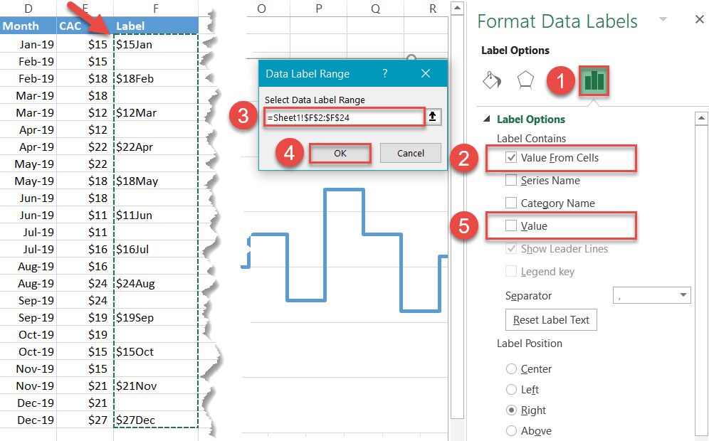
Remove data labels from excel chart. How to add or remove data labels with a click - Goodly Step 1) Add the Dummy values to the chart Note few things The data labels are turned - ON The 2 products (dummy calculations) are added on the primary axis See this - If you don't know how to add values to the chart Step 2) Place the dummy on the secondary axis Select the 2 data series (one by one) and use CTRL + 1 to open format data series box Excel Chart Data Labels - Microsoft Community Please verify that the range of data labels has been selected correctly. Right-click a data point on your chart, from the context menu choose Format Data Labels ..., choose Label Options > Label Contains Value from Cells > Select Range. In the Data Label Range dialog box, verify that the range includes all 26 cells. How to Change Excel Chart Data Labels to Custom Values? First add data labels to the chart (Layout Ribbon > Data Labels) Define the new data label values in a bunch of cells, like this: Now, click on any data label. This will select "all" data labels. Now click once again. At this point excel will select only one data label. Go to Formula bar, press = and point to the cell where the data label ... How to suppress 0 values in an Excel chart | TechRepublic Select the data set (in this case, it's B2:D9) Click Find & Select in the Editing group on the Home tab, and choose Replace. In Excel 2003, choose Replace from the Edit menu. In all versions, you...

How to remove a legend label without removing the data series In Excel 2016 it is same, but you need to click twice. - Click the legend to select total legend - Then click on the specific legend which you want to remove. - And then press DELETE. If my reply answers your question then please mark as "Answer", it would help others to find their solution easily from your experience. Thanks Report abuse Enable or Disable Excel Data Labels at the click of a button - How To Select and to go Insert tab > Charts group > Click column charts button > click 2D column chart. This will insert a new chart in the worksheet. Step 2: Having chart selected go to design tab > click add chart element button > hover over data labels > click outside end or whatever you feel fit. This will enable the data labels for the chart. How to Use Cell Values for Excel Chart Labels Select the chart, choose the "Chart Elements" option, click the "Data Labels" arrow, and then "More Options.". Uncheck the "Value" box and check the "Value From Cells" box. Select cells C2:C6 to use for the data label range and then click the "OK" button. The values from these cells are now used for the chart data labels. Create Excel Waterfall Chart Template - Download Free Template 09.06.2022 · Change Chart Title to “Free Cash Flow.” Remove gridlines and chart borders to clean up the waterfall chart. Step 3 – Add Data Labels to the Bars and Columns. Recall that we created a column called Data label position; this column will be used to define the position of the labels. Right-click on the waterfall chart and go to Select Data ...

Excel Pivot Table Report - Clear All, Remove Filters, Select … 9. Sort Data in a Pivot Table Report - Sort Row & Column Labels, Sort Data in Values Area, Use Custom Lists. 10. Pivot Table Report Layout, Compact, Outline and Tabular Form, Pivot Table Styles and Style Options, Design tab. 11. Pivot Chart Report: Create, Clear and Delete a Pivot Chart report, Pivot Chart Filter Pane, Pivot Chart and Regular ... Add or remove data labels in a chart - support.microsoft.com Data labels make a chart easier to understand because they show details about a data series or its individual data points. For example, in the pie chart below, without the data labels it would be difficult to tell that coffee was 38% of total sales. Depending on what you want to highlight on a chart, you can add labels to one series, all the ... How to Map Data in Excel (2 Easy Methods) - ExcelDemy First of all, select the range of the dataset as shown below. Next, go to the Insert tab from your ribbon. Then, select Maps from the Charts group. Now, select the Filled Map icon from the drop-down list. As a result, you will get the following map chart of countries. How to Use Cell Values for Excel Chart Labels 12.03.2020 · Make your chart labels in Microsoft Excel dynamic by linking them to cell values. When the data changes, the chart labels automatically update. In this article, we explore how to make both your chart title and the chart data labels dynamic. We have the sample data below with product sales and the difference in last month’s sales.

34 How To Label A Column In Excel - Labels Information List

Create Dynamic Chart Data Labels with Slicers - Excel Campus 09.02.2016 · Typically a chart will display data labels based on the underlying source data for the chart. In Excel 2013 a new feature called “Value from Cells” was introduced. This feature allows us to specify the a range that we want to use for the labels. Since our data labels will change between a currency ($) and percentage (%) formats, we need a ...

Enable or Disable Excel Data Labels at the click of a button - How To - PakAccountants.com

How to wrap X axis labels in a chart in Excel? - ExtendOffice When the chart area is not wide enough to show it's X axis labels in Excel, all the axis labels will be rotated and slanted in Excel. Some users may think of wrapping the axis labels and letting them show in more than one line. Actually, there are a couple of tricks to warp X axis labels in a chart in Excel. Wrap X axis labels with adding hard ...

How to insert data labels to a Pie chart in Excel 2013 - YouTube

How to add or move data labels in Excel chart? - ExtendOffice In Excel 2013 or 2016. 1. Click the chart to show the Chart Elements button . 2. Then click the Chart Elements, and check Data Labels, then you can click the arrow to choose an option about the data labels in the sub menu. See screenshot: In Excel 2010 or 2007. 1. click on the chart to show the Layout tab in the Chart Tools group. See ...

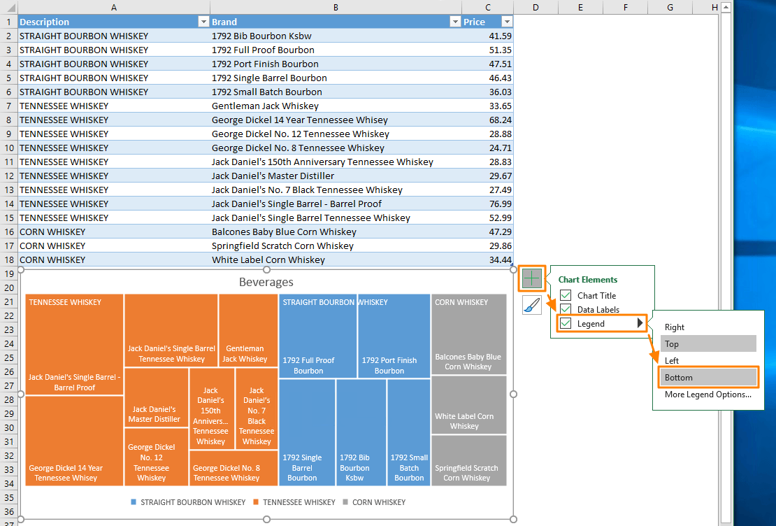
Treemap Excel Charts: The Perfect Tool for Displaying Hierarchical Data

Format Data Labels in Excel- Instructions - TeachUcomp, Inc. To format data labels in Excel, choose the set of data labels to format. To do this, click the "Format" tab within the "Chart Tools" contextual tab in the Ribbon. Then select the data labels to format from the "Chart Elements" drop-down in the "Current Selection" button group. Then click the "Format Selection" button that ...

Chart's Data Series in Excel - Easy Excel Tutorial

How to Create a Milestone Chart in Excel Steps to Create a Milestone Chart in Excel. I have split the entire process into three steps to make it easy for you to understand. 1. Set Up Data. You can easily set up your data for this chart. Make sure to arrange your data like below data table.

Enable or Disable Excel Data Labels at the click of a button - How To - PakAccountants.com

Prevent Overlapping Data Labels in Excel Charts - Peltier Tech Apply Data Labels to Charts on Active Sheet, and Correct Overlaps Can be called using Alt+F8 ApplySlopeChartDataLabelsToChart (cht As Chart) Apply Data Labels to Chart cht Called by other code, e.g., ApplySlopeChartDataLabelsToActiveChart FixTheseLabels (cht As Chart, iPoint As Long, LabelPosition As XlDataLabelPosition)

Excel Variance Charts: Making Awesome Actual vs Target Or Budget Graphs - How To ...

excel - Remove data label if less than a value - Stack Overflow What you need to do is remove the DataLabel for the specific point on the series. This should do it: Dim cht As Chart Set cht = ActiveChart If Range ("B8") < 0.01 Then cht.SeriesCollection (1).Points (1).DataLabel.Delete End If SeriesCollection (1) is the first series in the chart. Points (1) is the first point on the chart.

33 How To Label Bar Graph In Excel

How to create Custom Data Labels in Excel Charts Create the chart as usual. Add default data labels. Click on each unwanted label (using slow double click) and delete it. Select each item where you want the custom label one at a time. Press F2 to move focus to the Formula editing box. Type the equal to sign. Now click on the cell which contains the appropriate label.

Excel Charts - Free Excel Tutorial

How to Remove PivotTable Fields from Pivot Charts To remove the Field items, select the Analyze tab under the PivotChart Tools section. In the Show/Hide section, click on Field Buttons. Once selected, the Fields are removed from the chart. This is a quick and easy way to neaten up your Pivot Charts and ensure that your reports are sleek and readable. Excel Tips & Tricks, Tips & Tricks business ...

SIWI » Advanced Charts in Excel 2007

How to Add and Remove Chart Elements in Excel Select the data, go to insert menu --> Charts --> Line Chart. 1: Add Data Label Element to The Chart To add the data labels to the chart, click on the plus sign and click on the data labels. This will ad the data labels on the top of each point. If you want to show data labels on the left, right, center, below, etc. click on the arrow sign.

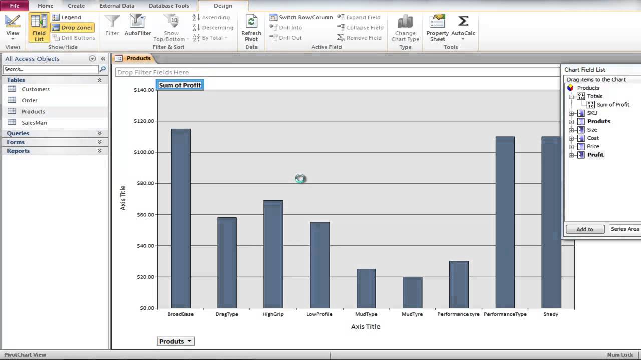
How to Create a Pivot Chart in Microsoft Access - YouTube

Change the format of data labels in a chart To get there, after adding your data labels, select the data label to format, and then click Chart Elements > Data Labels > More Options. To go to the appropriate area, click one of the four icons ( Fill & Line, Effects, Size & Properties ( Layout & Properties in Outlook or Word), or Label Options) shown here.

Charting in Excel - Adding Data Labels - YouTube

Excel 2010 Remove Data Labels from a Chart - YouTube How to Remove Data Labels from a Chart

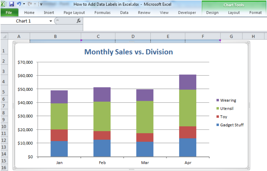
How to Add Data Labels in Excel - Excelchat | Excelchat

How to remove a bar from a bar chart - Microsoft Tech Community This is simple - I have a bar chart with 4 rows and 2 columns with a legend - I want to remove one of the rows - when I do this in the data sheet, the bars gets deleted but there is blank space left and I can't get rid of the space.

How-to Use Data Labels from a Range in an Excel Chart - Excel Dashboard Templates

Edit titles or data labels in a chart - support.microsoft.com Links between titles or data labels and corresponding worksheet cells are broken when you edit their contents in the chart. To automatically update titles or data labels with changes that you make on the worksheet, you must reestablish the link between the titles or data labels and the corresponding worksheet cells. For data labels, you can ...

How to Create a Step Chart in Excel - Automate Excel

MS Excel 2010 / How to remove data labels from the chart MS Excel 2010 / How to remove data labels from the chart1. Select chart object2. Go to Layout tab3. Click Data Labels button4. ... MS Excel 2010 / How to remove data labels from the chart1. Select ...

Share :