43 excel chart edit axis labels

Chart.Axes method (Excel) | Microsoft Docs This example adds an axis label to the category axis on Chart1. VB. With Charts ("Chart1").Axes (xlCategory) .HasTitle = True .AxisTitle.Text = "July Sales" End With. This example turns off major gridlines for the category axis on Chart1. VB. Excel Waterfall Chart: How to Create One That Doesn't Suck Click inside the data table, go to " Insert " tab and click " Insert Waterfall Chart " and then click on the chart. Voila: OK, technically this is a waterfall chart, but it's not exactly what we hoped for. In the legend we see Excel 2016 has 3 types of columns in a waterfall chart: Increase. Decrease.

Format Chart Axis in Excel - Axis Options Analyzing Format Axis Pane. Right-click on the Vertical Axis of this chart and select the "Format Axis" option from the shortcut menu. This will open up the format axis pane at the right of your excel interface. Thereafter, Axis options and Text options are the two sub panes of the format axis pane.

Excel chart edit axis labels

How to Change the X-Axis in Excel - Alphr Open the Excel file with the chart you want to adjust. Right-click the X-axis in the chart you want to change. That will allow you to edit the X-axis specifically. Then, click on Select Data. Next ... How to Format Chart Axis to Percentage in Excel? Select the axis by left-clicking on it. 2. Right-click on the axis. 3. Select the Format Axis option. 4. The Format Axis dialog box appears. In this go to the Number tab and expand it. Change the Category to Percentage and on doing so the axis data points will now be shown in the form of percentages. Change Text In Axis Of Chart In Excel Here I will introduce 4 ways to change labels' font color and size in a selected axis of chart in Excel easily. If we want to change the axis scale we should: Select the axis that we want to edit by left-clicking on the axis Right-click and choose Format Axis Under Axis Options, we can choose minimum and maximum scale and scale units measure.

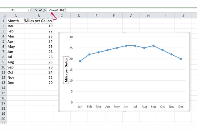
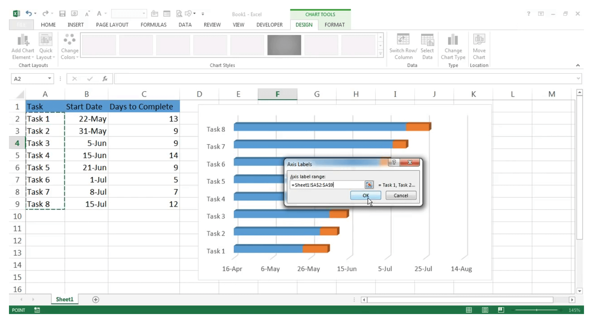
Excel chart edit axis labels. Use defined names to automatically update a chart range - Office On the Insert tab, click a chart, and then click a chart type. Click the Design tab, click the Select Data in the Data group. Under Legend Entries (Series), click Edit. In the Series values box, type =Sheet1!Sales, and then click OK. Under Horizontal (Category) Axis Labels, click Edit. In the Axis label range box, type =Sheet1!Date, and then ... Modifying Axis Scale Labels (Microsoft Excel) Follow these steps: Create your chart as you normally would. Double-click the axis you want to scale. You should see the Format Axis dialog box. (If double-clicking doesn't work, right-click the axis and choose Format Axis from the resulting Context menu.) Make sure the Number tab is displayed. (See Figure 1.) How to Add Axis Titles in a Microsoft Excel Chart Select the chart and go to the Chart Design tab. Click the Add Chart Element drop-down arrow, move your cursor to Axis Titles, and deselect "Primary Horizontal," "Primary Vertical," or both. In Excel on Windows, you can also click the Chart Elements icon and uncheck the box for Axis Titles to remove them both. If you want to keep one ... Exactly How to Add Axis Titles in a Microsoft Excel Chart Click the Add Chart Element drop-down arrow and also move your arrow to Axis Titles. In the pop-out food selection, choose "Primary Horizontal," "Primary Vertical," or both. If you're making use of Excel on Windows, you can also make use of the Chart Elements symbol on the right of the chart. Check the box for Axis Titles, click the ...

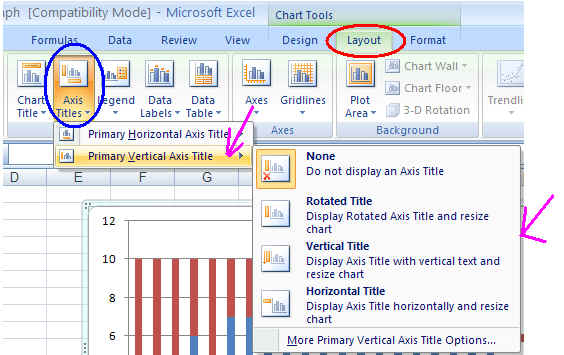
How to make shading on Excel chart and move x axis labels to the bottom ... In the text options for the horizontal axis, specify a custom angle of -45 degress (or whichever value you prefer): For the yellow shading, add a series with constant value -80, and a series with constant value -20. In the Change Chart Type dialog, change the chart type for the new series to Stacked Area. Modifying Axis Scale Labels (Microsoft Excel) - tips You can very easily change the axis scale by simply modifying how the values on the axis are displayed. Follow these steps: ... Excel 2002, and Excel 2003: Create your chart as you normally would. Double-click the axis you want to scale. You should see the Format Axis dialog box. ... Double-click on the Thousands label to edit the label, as ... How to Change Axis Scales in Excel Plots (With Examples) Step 3: Change the Axis Scales. By default, Excel will choose a scale for the x-axis and y-axis that ranges roughly from the minimum to maximum values in each column. In this example, we can see that the x-axis ranges from 0 to 20 and the y-axis ranges from 0 to 30. To change the scale of the x-axis, simply right click on any of the values on ... How to Add Axis Label to Chart in Excel - Sheetaki Method 1: By Using the Chart Toolbar. Select the chart that you want to add an axis label. Next, head over to the Chart tab. Click on the Axis Titles. Navigate through Primary Horizontal Axis Title > Title Below Axis. An Edit Title dialog box will appear. In this case, we will input "Month" as the horizontal axis label. Next, click OK. You ...

How to use Axis labels in Excel - PapertrailAPI Type the axis title. 5. To link the axis title with text from a cell, go to the formula bar and type = after step 3. Click on the cell with axis label text ( A1 ). 6. Press ENTER. The text 'Axis Tile' will update to the text in the selected cell ( Day ). 7. To add y-axis title, click on the chart of interest. How to Create and Customize a Waterfall Chart in Microsoft Excel Select the chart and use the buttons on the right (Excel on Windows) to adjust Chart Elements like labels and the legend, or Chart Styles to pick a theme or color scheme. Select the chart and go to the Chart Design tab. Then, use the tools in the ribbon to select a different layout, change the colors, pick a new style, or adjust your data ... How to Change the Y Axis in Excel - Alphr To change the axis label's position, go to the "Labels" section. Click the dropdown next to "Label Position," then make your selection. Changing the Display of Axes in Excel Can't edit charts - all options greyed out - Microsoft Tech Community Hi - I've recently been upgraded to Office 365. I've got a regular reporting spreadsheet, with charts that need updating. However, I can't edit any of the charts! I can't right click anywhere on the sheets containing the charts, and all the options on the 'Chart Design' and 'Format' ribbon tabs are greyed out.

How to Add an Axis Title to an Excel Chart | Techwalla

Excel - 2-D Bar Chart - Change horizontal axis labels I have a 2-D bar chart in Excel. I want to change the horizontal axis labels to be different from the data. Editing the Data Source only changes the vertical axis labels, not the horizontal labels ...

Help Online - Origin Help - The Tick Labels Tab

How to format axis labels individually in Excel - SpreadsheetWeb Double-click on the axis you want to format. Double-clicking opens the right panel where you can format your axis. Open the Axis Options section if it isn't active. You can find the number formatting selection under Number section. Select Custom item in the Category list. Type your code into the Format Code box and click Add button.

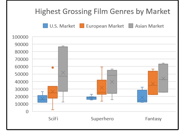
What to do with Excel 2016's new chart styles: Treemap, Sunburst, and Box & Whisker | PCWorld

How To Change Symbols On Excel Graph? New Update Step 1: Accessing Symbols in Excel. Select an empty cell to insert the symbols into. Go to the Insert tab in the ribbon. From the Symbols section, press the Symbol button. Select Arial from the Font drop down list. Select Geometric Shapes from the Subset drop down list. Select the arrow.

ABC Inventory Analysis using Excel Charts - PakAccountants.com

Controlling Chart Gridlines (Microsoft Excel) Instead, you can control the gridlines by following these steps: Select the chart by clicking on it. You should see selection handles appear around the outside of the chart. Make sure that the Format tab of the ribbon is displayed. (This tab is only visible when you've selected the chart in step 1.) In the Current Selection group, use the drop ...

EXCEL GRAPHING

Excel: How to Create a Bubble Chart with Labels - Statology Step 3: Add Labels. To add labels to the bubble chart, click anywhere on the chart and then click the green plus "+" sign in the top right corner. Then click the arrow next to Data Labels and then click More Options in the dropdown menu: In the panel that appears on the right side of the screen, check the box next to Value From Cells within ...

How to Make Gantt Chart in Excel? | Gantt Chart Excel - Zoho Projects

Pivot chart X axis labels not aligned to the ... - Excel Help Forum Re: Pivot chart X axis labels not aligned to the corresponding vertical bars. I may not be the best one to walk you through the steps, since my older version of Excel might use a different interface. Basically: 1) Select either data series (I selected one of the orange bars). 2) Bring up the "format data series" dialog/pane (see if this help ...

Excel Course: Inserting Graphs

Change Text In Axis Of Chart In Excel Here I will introduce 4 ways to change labels' font color and size in a selected axis of chart in Excel easily. If we want to change the axis scale we should: Select the axis that we want to edit by left-clicking on the axis Right-click and choose Format Axis Under Axis Options, we can choose minimum and maximum scale and scale units measure.

Legend help

How to Format Chart Axis to Percentage in Excel? Select the axis by left-clicking on it. 2. Right-click on the axis. 3. Select the Format Axis option. 4. The Format Axis dialog box appears. In this go to the Number tab and expand it. Change the Category to Percentage and on doing so the axis data points will now be shown in the form of percentages.

Share :